
Quasi-Bayesian Inference for Grouped Panels
Last Update:
Why Quasi-Bayesian Clustering?
There are two popular methods to recover latent group structure:
Frequentist clustering is given by
\[(\hat{\boldsymbol{\beta}},\hat{\boldsymbol{\gamma}}) = \arg\min \overline{L}(\boldsymbol{\beta},\boldsymbol{\gamma})\]- $\overline{L}(\boldsymbol{\beta},\boldsymbol{\gamma})$ is a sample loss function, for example, least squares
- loss function specification is flexible and robust to model misspecification, compared to full data likelihood
- but measuring uncertainty in \(\boldsymbol{\gamma}\) is difficult
Bayesian clustering is characterized by the posterior 1
\[\pi_{NT}(\boldsymbol{\beta},\boldsymbol{\gamma})\propto \pi(\mathbf{W}|\boldsymbol{\beta},\boldsymbol{\gamma}) \pi(\boldsymbol{\beta},\boldsymbol{\gamma})\]- \(\pi(\boldsymbol{W}\mid\boldsymbol{\beta},\boldsymbol{\gamma})\) is the likelihood and \(\pi(\boldsymbol{\beta},\boldsymbol{\gamma})\) a prior, for example, mixture prior on \(\boldsymbol{\gamma}\) and normal prior on \(\boldsymbol{\beta}\)
- straightforward to quantify uncertainty in the group structure \(\boldsymbol{\gamma}\)
- but specifying the full data distribution, i.e., the likelihood, can be difficult
The idea of quasi-Bayesian clustering is to combine the loss component and the prior component, leading to the quasi-posterior:
\[\pi_{NT}(\boldsymbol{\beta},\boldsymbol{\gamma}) \propto \left( \exp \left[ -NT\; \overline{L}(\boldsymbol{\beta},\boldsymbol{\gamma})\right] \right)^{ \psi} \pi(\boldsymbol{\beta},\boldsymbol{\gamma})\]Here, we have an additional learning rate parameter $\psi$, which controls the relative weight on the loss component. In plain words, it determines how much we learn from the data (relative to prior knowledge).
Learning Rate Calibration
One key feature of the quasi-Bayesian clustering framework is the learning rate calibration. To see how this learning rate can improve inference, I show below the quasi-posterior densities of two bootstrapped samples, under different learning rates.
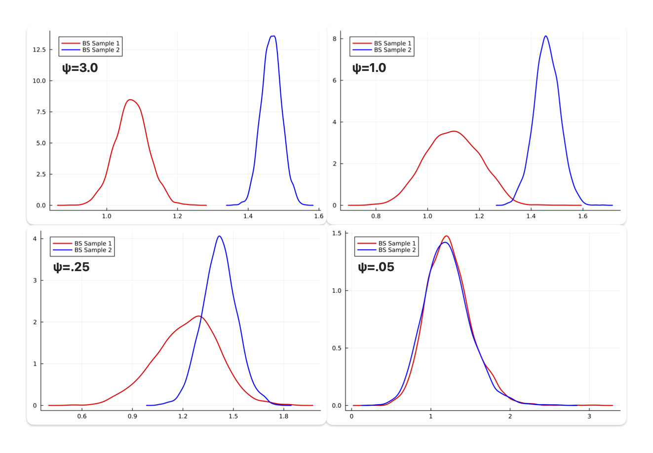
- When learning rate is large (say, $\psi=3.0$), the quasi-posterior puts a large weight on the loss component, and thus suffer from selection bias (as shown by different posterior modes) while the variance is relative low (the posterior densities are quite concentrated)
- As the learning rate gets smaller, the two posteriors get closer and closer—the posterior modes are closer to the true, at the expense of larger variance (the quasi-posteriors are more dispersed)
- Ideally, we would calibrate the learning rate to a point where bootstrapped samples give identical posterior distributions (as the bottom right panel $\psi=0.05$ shows), while keeping the variance as small as possible
Another likelihood-based clustering method is finite mixture models, usually estimated by efficient EM algorithm. Like Bayesian methods, it requires the likelihood to be correctly specified. ↩